The Black-Scholes Magic Trick, Explained!

The economist Paul Romer once compared the models used in finance with the tricks used by magicians, whose secrets are protected by the Magician’s Oath. As he wrote in 2015, “A model is like doing a card trick … Perhaps our norms will soon be like those in professional magic; it will be impolite, perhaps even an ethical breach, to reveal how someone’s trick works.” [Spoiler alert: guilty as charged.]

Of course, nothing can be kept secret forever, so once a magician has invented something like a levitation trick, as illusionists did some two centuries ago, other versions soon follow. Today, you can find explanations on YouTube, or Wikipedia. But for most audiences, the trick will still be effective.

An example of such a mathemagical trick is the Black-Scholes model, which since its publication in 1973 has served as the industry-standard model used to price financial options – those instruments which give one the right but not the obligation to buy (a call option) or sell (a put option) a stock in the future at a set price, known as the strike. The model is magically simple: in order for the price of the option to be revealed, traders only need to supply two key pieces of information: the risk-free interest rate, which can be obtained from something like a Treasury bond, and the volatility, which is an estimate of price variation (technically, it is the standard deviation of the logarithm of price changes over a period such as a year).

As financial magic shows go, the Black-Scholes model has certainly had a good run – one of the longest on Wall Street, and elsewhere – and has received rave reviews. One commentator (Ross, 1987) described option pricing as “the most successful theory not only in finance, but in all of economics.” Another (Rubinstein, 1994) said the algorithm may be “the most widely used formula, with embedded probabilities, in human history.” Even critics acknowledge the model’s importance to the field; Nassim Nicholas Taleb (1998) wrote that “Most everything that has been developed in modern finance since 1973 is but a footnote,” while in his 2008 report to shareholders Warren Buffet said it had “approached the status of holy writ” (magic being closely related to religion).

A popular component of magic shows is the prediction trick, where the magician makes a seemingly impossible prediction about an audience member or something else. The Black-Scholes formula does this but with a twist. Its trick is to present itself, not so much as a prediction, but rather as a magical machine which somehow defines the correct option price – like a mentalist who predicts the future by making it happen. And by using the machine as a calculating device, investors only seem to confirm its predictions. What kind of higher-level voodoo is this?

Such is its hypnotic hold, that it defines the very words and concepts used by quants to describe option pricing. For example there is the “implied volatility” which is the special number that must be fed into the machine in order for it to work, but whose true value can be divined only in hindsight. And then there are the “Greeks” which refer to various terms thought to describe its sensitivities, and are reminiscent of the arcane symbols employed by sorcerers. For example the symbol Δ shows how the option price depends on the current asset price, while Θ measures its dependence on time.

Even more remarkable is that the mesmerising power of the model’s spell has distracted the audience from worrying about – or often even noticing – the fact that its assumptions have no more obvious means of support than a magician’s levitating assistant.

Suspending disbelief

For example, one of its totems is that markets are “efficient” so are made up of what economist Eugene Fama (1965) called “rational profit maximizers” whose collective actions ensure that everything is priced rationally, including assets and options. If anyone still think markets are rational and efficient, then see below.

Much of the power of the model comes from its amazing use of “dynamic hedging” which assumes that someone can constantly buy and sell options and the underlying stock in such a way that the risks are always balanced. The theory appears to mathematically prove that the value of an option does not depend on the growth of the underlying asset (which is why the formula uses only the risk-free rate). And yet it obviously kind of does, which is why for something like the S&P 500 index, which tends to grow, call options (to buy) have consistently outperformed put options (to sell). This is a problem, since the test of the model is not to satisfy some abstract theorem, or even to predict what traders are paying for options; it is to predict what prices correspond to the expected payouts.

The model assumes that prices follow a “random walk”, so the probability distribution for price changes should be lognormal (i.e. the log price changes should follow a bell curve). But, it’s not. It has “fat tails” meaning that the chances of extreme price changes, such as a crash or a spike, are much higher than predicted by the model.

The model also assumes that volatility over a set period can be treated as constant, and in particular does not depend on the strike, which again is the reference price for the option. But if you plot volatility versus price change for historic asset price data it turns out that there is a distinct smile shape, with volatility lower for periods over which the price change is small, and climbing higher as the price change becomes increasingly positive or negative. (Note that price change is clearly related to the strike price, since options with different strikes can be viewed as the same option with a corresponding assumed price change.) A similar “volatility smile”, though somewhat less pronounced, is seen when the implied volatility used by traders is plotted versus strike – a clue left in plain sight.

The markets are smiling, but Black-Scholes doesn’t get the joke. Figure shows plots of volatility over time periods of 1, 2, 4 and 8 weeks (light to dark), for the S&P 500 index (1992-2022), compared with a prediction using a quantum model (dashed). The horizontal axis is price change x normalised by the square-root of time T. The Black-Scholes formula assumes volatility is constant so these lines are all flat.

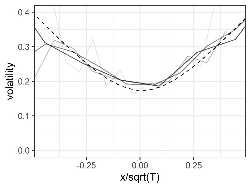
Finally, that dynamic hedging proof, which in a wave of its magic wand appeared to remove the dependence on subjective estimates of future growth, demands that you can constantly buy and sell securities and options to eliminate risk. This ignores the bid-ask spread (the difference between the buyer price and the seller price) on those transactions – which is not a technical detail, but represents a level of irreducible uncertainty, whose magnitude is related to the volatility. Include those, and the clarity, certainty, and elegance of the mathematical demonstration loses some of its theatrical sparkle. (The dashed line in the above figure was derived from a quantum economics model, which uses a different kind of magic.)

How to be beaten by the market

Now, most people in the audience will be untroubled by these details – or won’t perceive them at all – because they will tell themselves that (a) the model has a great back story and is rooted in highly rational mathematics, and (b) what ultimately counts is that the magic formula is widely known to give the “right” answers (i.e. correct predictions of the fair price), at least if we set aside the occasional stage malfunction such as the 1987 Black Monday crash, the 1998 LTCM blow-up, the 2007/8 financial crisis, and so on, where use of the model led to large losses. (Advocates of efficient market theory can explain all of these, thus falsifying the theory that theories in finance can ever be falsified.) Any nagging doubts can be addressed by inventing elaborate excuses, or by noting that no model is perfect, the Black-Scholes model has the advantage of simplicity, it is very useful as a mental tool, traders adjust the price anyway, and so on.

Only, the model doesn’t give the right answers, its predictions are off, the crystal ball is cracked. Here’s another clue: suppose you agreed to buy lots and lots of 1-month at-the-money S&P 500 straddle options (a combination of a call and a put), at the price suggested by the model using the benchmark (VIX index) volatility, and kept reinvesting the takings. If markets are efficient, and the model is telling the truth, then in principle you should expect to break even over a sufficiently long period of time. Except you won’t, you’ll lose money, in an efficient manner (this is not financial advice). In fact, you would overpay by a factor about equal to the square-root of two.

Losses will be reduced if you pay the actual market price for these options, since traders feed the oracle a lower volatility number, but they will still be significant, which again seems to contradict the efficient market hypothesis. The reason is that volatility, which is the mysterious essence at the heart of the trick, isn’t actually a thing, at least in the sense assumed by the formula. You can measure price changes over a previous period and calculate a standard deviation. Since conditions are always changing, the answer you get will depend on the exact period, so you might try to adjust for this somehow. But if the future variability is itself a highly variable quantity which depends, like expected price change, on the state of the market, then there is no single volatility that is independent of strike.

Also, since dynamic hedging isn’t a thing either, the assumption that the growth rate equals the risk-free rate – with no need for subjective estimates or uncertain predictions – is itself just a particular choice or prediction, and one which is not backed up by empirical data. The whole carefully-constructed illusion of deterministic objective rationality shatters into pieces.

All this won’t spoil the entertainment as long as people don’t look too hard behind the scenes, or check what’s going on using actual statistical tests (there being more data now than in 1973). But this still leaves the question of how this trick works. How does it get so many people to take the word of an elegant but obviously idealised mathematical proof, instead of confirming whether option prices correspond to expected payouts, which is the normal test for a statistical predictive model? Or to go along with the idea that the volatility smile is a puzzling anomaly or “logical inconsistency” (as it has been called) caused by market quirks, or irrational behaviour on the part of traders, instead of being a reflection of a real phenomenon? And how does a square-root of two error get magicked out of existence?

The logic hack

Part of the reason for the trick’s success is that, as already mentioned, it substitutes the usual test of a model, which is to predict outcomes, with a different test, which is to obey an abstract proof based on certain assumptions, thus again rendering it unfalsifiable. But at a deeper level, the secret behind the trick is that it induces in its audience what might be described as model blindness. As quants Emanuel Derman and Michael Miller (2016) note, the model “sounds so rational, and has such a strong grip on everyone’s imagination, that even people who don’t believe in its assumptions nevertheless use it to quote prices at which they are willing to trade.” By hacking (like a hypnotist on a hapless showgoer) into people’s ideas about rationality, it changes their perception of reality, and even the language they use to describe it, so the model’s word takes precedence over observable facts (the smirking volatility, the money-losing options). Which is quite a mind-blowing stunt.

Of course, like most tricks it wouldn’t have worked if the people in the gallery hadn’t at some level wanted it to work. But the real audience back in the 1970s, when it first came out, wasn’t just options traders – it was society as a whole. The illusion of predictability, objectivity and rationality was at the time in a sense necessary and productive, because it transformed options trading from a slightly disreputable form of gambling, into scientific risk management, and thus helped conjure into existence much of the quantitative finance industry. A shared language acted as a coordination device which allowed traders to communicate and do business. The audience was therefore part of the performance, and shared in the magical profits (one could even say that they, more than the inventors themselves, were the magicians who made the trick work). And it was all just one component in an even longer-running magic show, which is the neoclassical illusion that the complex, unstable, living system known as the economy is actually a rational, efficient, utility-maximising machine. Magicians have traditionally tried to convince people that the automaton is alive, but here it is the other way round.

The Black-Scholes model is one of the greatest mathemagical tricks of all time. But now, it might be time for us to snap out of this illusion, open our eyes, and let go of this idea that markets are efficient and obey rational logic. After all, it always did sound a little crazy.

An earlier version of this article appeared in the July 2023 issue of Wilmott Magazine.

The Prediction Test

The two most famous theories in the field of forecasting are the butterfly effect, and the efficient market hypothesis. Both are theories, not of prediction, but of non-prediction.

The butterfly effect was developed by MIT meteorologist and chaos theorist Ed Lorenz in the 1960s. He found that computer simulations of a toy weather model tended to stray apart over time if the starting point was changed by even a tiny amount (chaos!). He proposed that this “sensitivity to initial condition” was a property, not just of his three-equation model, but of the weather itself. When he submitted an untitled talk for the 1972 conference of the American Association for the Advancement of Science, the person hosting the session supplied a provocative title: “Predictability; Does the Flap of a Butterfly’s Wings in Brazil Set Off a Tornado in Texas?”

The efficient market hypothesis was first proposed in a 1970 PhD thesis by Eugene Fama, from the University of Chicago. It says that price changes in financial markets are caused by random perturbations (e.g. news) and therefore follow a “random walk” which is inherently unpredictable.

Apart from fame, the theories have many other things in common. They both provide a scientific reason for forecast errors, such as the financial crisis. They both assume that forecast error is due to random effects (insects or news). Both theories – or at least their typical applications – assume that the underlying model of the system is correct. And they are both used to justify complicated techniques that are hard to interpret or falsify.

In the 1990s weather forecasters seized on the butterfly effect as an excuse for forecast error, but also as a rationale for elaborate “ensemble forecasting” schemes. Instead of making a single “point” forecast, an ensemble of forecasts is here generated from a set of perturbed initial conditions, and used to produce a statistical forecast that takes into account the effects of chaos. When forecasters made typical perturbations of the sort that might be produced by observational error, they found that the simulations didn’t diverge as quickly as expected, which was possibly a hint; however they soon found ways to select specially optimised perturbations which did exhibit the desired divergent behaviour.

The efficient market hypothesis meanwhile might have shown that price changes were unpredictable, but also enabled the use of statistical models which claimed to predict the probability of a price change, such as the Value at Risk model. In either case of course the statistical forecast is only valid if the underlying model of the system is correct.

Both theories are hard to disprove, and remarkably resilient to criticism. When I (David) showed in a 1999 presentation at the European Centre for Medium-Range Weather Forecasts that plots of forecast error show a square-root shape, which is characteristic not of chaos but of model error, I was contradicted by a number of people in the audience. The next day I received an email from one of the top research heads, which said that he had checked a plot of forecast errors, and, in stark contrast to my talk, “they certainly show positive curvature.” In other words, they were caused by chaos, not model error. We therefore decided that someone there should try to reproduce my results, by plotting the errors as a function of time.

When the results showed a near-perfect square-root shape, I received an email saying that “I guess it would be possible to get an initially square root shape from initial condition error if the error was initially in very very small scales which rapidly saturates but cascades up  to produce errors of larger scale, which then saturate, but cascade up to produce errors of still larger scale.” (That was the exact point when my view of science began to shift.)

Similarly, as Andrew W. Lo and A. Craig MacKinlay wrote in their book A Non-Random Walk Down Wall Street: “One of the most common reactions to our early research was surprise and disbelief. Indeed, when we first presented our rejection of the Random Walk Hypothesis at an academic conference in 1986, our discussant – a distinguished economist and senior member of the profession – asserted with great confidence that we had made a programming error, for if our results were correct, this would imply tremendous profit opportunities in the stock market. Being too timid (and too junior) at the time, we responded weakly that our programming was quite solid thank you, and the ensuing debate quickly degenerated thereafter. Fortunately, others were able to replicate our findings exactly.”

Needless to say, both the butterfly effect and efficient market theory survived these and other challenges.

Finally, both theories rely on a kind of magical thinking – that the atmosphere is incredibly sensitive to the smallest change, so perturbations grow exponentially instead of just dissipating (try waving your hand in front of your face to see which is more physically realistic); or that the economy is magically self-correcting, like a door which snaps instantly shut after being opened.

One difference is that the butterfly effect does double duty in other areas such as economics. As then-Fed chairman Ben Bernanke explained in 2009, “a small cause – the flapping of a butterfly’s wings in Brazil – might conceivably have a disproportionately large effect – a typhoon in the Pacific” which was a useful thing to bring up after you just failed to predict the US housing crisis. However, the idea that unpredictability is caused by efficiency has failed to catch on outside of economics. For example, no one thinks that snow storms that come out of nowhere are efficient.

So why are these theories both still around? The reason is simple. As the physicist Richard Feynman once said, “The test of science is its ability to predict.” The magic of science is the ability to make it look like you can predict.

Swingers

This post looks at Mathematical Thinking, which we define as “The belief, especially characteristic of scientists, that events can be understood, described, and predicted using mathematical equations; thinking founded on this belief.” Sometimes it’s a good thing, sometimes not so good.

Imagine you’re at the bar, and order a gin martini. The bar man serves it in the usual conical martini glass. Tell us, when the drink is halfway down the side of the glass how much is left?

Half? No, the glass is pointy at the bottom so there’s clearly less in the bottom half than in the top half. A quarter? Final answer. One quarter!

Wrong.

You may recall from school the idea of similar triangles. They are triangles with the same shape, but a different size. This is what we also see in the cone, our martini glass. The bottom half of the martini glass is “similar” to the full glass.

The problem of calculating volumes of geometric objects goes back to the ancient Greeks. Draw a square on a piece of paper and then draw another with sides twice the length. How much has the area increased by? It’s four times bigger. You can see that four of the smaller squares will fit inside the larger. Now take eight sugar cubes or dice. Put four into a square and put another four on top. You’ve now got a larger cube, each side of which is twice the length of the smaller. So for a cube halve the length, you’ve got a volume that’s a mere eighth of the original!

The shape doesn’t matter here. All that matters is that the half-full glass is “similar” in the mathematical sense to the full glass. The formula is just 1 divided by 2 raised to the power d, where d is the number of dimensions. Since we live in d = 3 dimensions – we’re leaving out spooky extra dimensions – the answer is 1 divided by 2 cubed, which is 1/8, or 12.5%.

Or in mathematical terms: it’s time to order another.

Mathematicians are full of tricks like this where pure thought can lead to answers that are not otherwise obvious or where the brain gets tricked. Say that, reaching for a bottle on an upper shelf behind the bar, the barman’s arm brushes against a light hanging from a cable, making it swing gently. What is the time taken to swing left to right then back again (i.e. the period)?

Galileo first became interested in this problem when he noticed the sway of a chandelier in the Pisa cathedral. There are a few ways of solving it mathematically. Most require some knowledge of physical laws, but there is a simple method known as dimensional analysis that gets you most of the way there. As the name suggests, it is again based on the concept of dimension.

We first ask what quantities could affect the period of the swing. A couple are obvious: the mass of the weight, and length of the string. Anything else? The colour of the string or the time of day shouldn’t come into it, but one can imagine the answer is different on the moon from here in the bar so gravity must play a role. The acceleration due to gravity, usually represented by g, is 9.8 meters per second squared. On the moon it is only about 16 percent of that number, because the moon is less massive.

Now let’s postulate that the period is given by multiplying or dividing those numbers together, where again you are allowed to raise a number to a power. We will include fractional powers, so for example a number raised to the power ½ is the square root. The trick is that, for the formula to work, the units of the expression of the period, which are seconds, have to be the same as the units of the expression that you just made up. The two sides of the equation must be made of the same stuff.

The two sides of an equation must be made of the same stuff.

Write it out and you find that the only way to make it work is if – ta da! – the period of the swing is proportional to the square root of length divided by the gravitational constant g. So the mass doesn’t – and can’t – come into it.

There is no magic involved here, no spooky automatic writing or communication with the other side, but in a sense the result is magical, because it shows us something very counterintuitive, namely that the time of the swing doesn’t depend on the mass of the pendulum. The weight only comes in through the acceleration due to gravity. On the moon gravity is less and the swing will take longer. In fact, you can use this relationship to test tiny local perturbations in the gravitational field.

It turns out that if the length is exactly one meter, then the period T is almost exactly 2 seconds, and a single swing counts out a second. Which is why traditional grandfather clocks, first produced in the late seventeenth century, have a pendulum of this length. It also inspired the definition of the metre a century later.

This technique of dimensional analysis has been used to great effect in other circumstances. New Mexico was the site of the first explosion of an atomic bomb, at 5:29am on July 16, 1945. Codenamed “Trinity,” much of the project – including the amount of energy released by the explosion – was obviously kept secret. However one observer at the explosion was the mathematician GI Taylor. Taylor is famous for his work in fluid and solid mechanics, in particular the difficult problem of turbulent flow. He estimated the energy in the atomic explosion by applying precisely the above dimensional trick but with quantities energy, air density, radius of the explosion, and time. He estimated the energy released to be 17 kilotons of TNT. President Truman later revealed it to have been 22 kilotons. Taylor’s approximation was remarkably accurate and shows the power of quite simple mathematics, or perhaps more precisely the power of Mathematical Thinking. As we’ll see, similar thinking was behind the bomb itself – this is a dangerous kind of power.

Few people are as clever as GI Taylor. And unfortunately there are many people as gullible as Doyle. But there is also an intersection between magical thinking and mathematical thinking where the power and beauty of mathematics gets used as a decoy to confound while giving the illusion of clarity. We first discovered this happening in finance and economics. But once you’ve been alerted to the possibilities of such abuse you start seeing examples everywhere.

This is what we call Mathemagical Thinking. And in the wrong hands it can be as dangerous as nuclear weapons.

Magos

Magic and science have a surprising amount in common. They are both about telling a story, and constructing a narrative of events. In one, the story appears magical, in the other it appears mathematical, but that difference is less important than might appear. They can both be dangerous if misapplied. In fact, one could argue that science is truer to the spirit of magic than most modern magicians are.

Back in ancient Greece, where the term originates, the magos (magicians) were religious figures, like shamans, who were believed to have access to the Otherworld. They performed rituals and ceremonies, administered healing potions, cast spells on enemies, or contacted the dead through seances. They were not usually connected to official temples – who viewed them with suspicion – but operated as freelancers, selling their services in the private market.

Such gnostics and mystics have throughout history operated on the fringes of mainstream religion – with “superstitions” instead of official sacraments, and “witchcraft” instead of sacred rites. But they still had considerable knowledge and power, and were far more than a source of entertainment. They didn’t do children’s parties. And the separation between magic and science was not so clear.

Pythagoras, who is sometimes described as the first pure mathematician, ran what amounted to a pseudo-religious cult with all kinds of strange teachings and an interest in esoteric symbols. The first mathematical models of the cosmos were developed by Greek mathematicians expressly for the purpose of reading the future through astrology. Chemistry grew out of alchemy, whose practitioners included scientists such as Isaac Newton. In the late nineteenth century, the discovery of the cathode ray tube, with its eery green glow, seemed to excite the spiritualist community as much as it did the scientific community (though that changed when it became the basis for TVs).

Even today, science is often as much about putting on a great show and amazing us with magical demonstrations as it is about making life-altering discoveries. Consider for example the moon landing of 1969 (though some claim it was a staged illusion) which was actually about impressing the Russians with military technology. Or more recently the excitement about the discovery of a tiny ghostlike particle known as the Higgs boson, which sounds like something a wizard would concoct.

Perhaps the main difference now is that magicians are seen as mere paid entertainers, while scientists are revealing the deep truths of the universe. Our aim in this blog is to break down this barrier to show the still-powerful connection between magic and science. Through a sequence of stories, historical nuggets, magic tricks, and other amusements, we reveal some of the tricks that scientists play on their audience. And we will show how even in the modern scientific age, many people are prone to mathemagical thinking.

Automatic Writing

On the topic of gullibility, here is a story that we like to share with our banker friends during our “seminars” on magical thinking (much better paid than real magic shows and the audience is less demanding).

In the summer of 1922, Sir Arthur Conan Doyle invited his friend, the magician Harry Houdini, and his wife Bess to join them for a week at Atlantic City. The vacation was going well, and everyone was having a good time, until Sir Arthur suggested that his wife Jean could put Houdini in touch with Houdini’s beloved mother Cecelia, who had died almost a decade earlier.

Sir Arthur was of course famous for being the creator of the ultimate scientific rationalist Sherlock Holmes, however he had also been converted to spiritualism after losing his son and brother during World War I. When he saw Houdini perform his act during a tour through England, he became convinced that Houdini had genuine supernatural powers. And he had great faith in his wife’s talent as a medium.

For Houdini, the situation was complicated. For one thing, he knew that his illusions were the product of stagecraft, not magic, and that Sir Arthur was overly gullible. He had also authored a book in which he revealed the tricks of a number of magicians and mediums. It was inspired in part by earlier, unsuccessful attempts to contact his mother, who he had seen as “the guiding beacon of my life.” But at the same time, he liked Doyle – and he really missed his mother. So he agreed to give it a go.

The séance was held at the Doyles’ hotel room. After turning down the lights, Lady Jean went into what appeared to be a deep trance. Then she grabbed a pen and started scribbling manicly on sheets of paper – what spiritualists called automatic writing – as if she were channeling the spirit of Houdini’s mother. Houdini read the sheets as she finished them, fifteen in all before she wound herself down. But his awkward feelings were not relieved.

The letter said all the usual things that one might expect from a long-dead mother (love you, missing you, the Doyles are great, etc.) but it was written in perfect English (his mother was Hungarian and spoke little English), the first sheet was decorated with a cross (she was a Jew), she didn’t mention that it was her birthday that day, and so on. He didn’t need to be Sherlock Holmes to realise he was being conned.

Not wanting to spoil the evening, or their relationship, he didn’t say anything at the time; but matters came to a head later that year when he wrote an article saying that no medium had ever been proven to be able to contact the dead. Evidence-based, they were not. Doyle took it personally, and the friendship was effectively over.

Doyle continued to write books and give lectures promoting spiritualism. Houdini remained a skeptic, but still held out some hope that it might be possible to communicate with the departed – being a magician didn’t make him completely immune to magical thinking. He arranged a code with his wife, so that if she tried to contact him after his death through a medium she would know whether it was genuine. After he died in 1926, of a ruptured appendix on Halloween, Bess kept trying, but to no avail. She finally stopped the séances in 1936, famously announcing that “ten years is long enough to wait for any man.”

By that time, the craze for spiritualism was already losing some of its energy. And today, of course, most people see séances as something from an earlier, less scientific age. We know that for many people the desire to communicate with lost relatives is so great that they are willing to suspend disbelief; and that doing so makes them susceptible to the con-artists and fraudsters who Houdini had worked to debunk. But that doesn’t mean that we are immune to the power of magic – even when we are trying to be rational.

Bankers (and others) beware.